Dichotomizing continuous predictors in multiple regression: a bad idea
STATISTICS IN MEDICINEStatist. Med. 2006; 25:127–141Published online 11 October 2005 in Wiley InterScience (www.interscience.wiley.com). DOI: 10.1002/sim.2331
Dichotomizing continuous predictors in multiple regression:
Patrick Royston1;∗;†, Douglas G. Altman2 and Willi Sauerbrei3
1MRC Clinical Trials Unit; 222 Euston Road; London NW1 2DA; U.K.
2Centre for Statistics in Medicine; University of Oxford; Wolfson College Annexe; Linton Road;
3Institute of Medical Biometry and Medical Informatics; University Hospital of Freiburg;
Stefan-Meier-Str. 25; 79104 Freiburg; Germany
In medical research, continuous variables are often converted into categorical variables by groupingvalues into two or more categories. We consider in detail issues pertaining to creating just two groups,a common approach in clinical research. We argue that the simplicity achieved is gained at a cost;dichotomization may create rather than avoid problems, notably a considerable loss of power andresidual confounding. In addition, the use of a data-derived ‘optimal’ cutpoint leads to serious bias. Weillustrate the impact of dichotomization of continuous predictor variables using as a detailed case studya randomized trial in primary biliary cirrhosis. Dichotomization of continuous data is unnecessary forstatistical analysis and in particular should not be applied to explanatory variables in regression models. Copyright ? 2005 John Wiley & Sons, Ltd.
continuous covariates; dichotomization; categorization; regression; e ciency; clinical
‘Why have researchers continued to ignore methodologists’ advice not to dichotomize theirmeasures?’ [1]. Measurements of continuous variables are made in all branches of medicine,aiding in the diagnosis and treatment of patients. In medical research, such continuousvariables are often converted into categorical variables by grouping values into two or morecategories. It seems that the usual approach in clinical and psychological research is todichotomize continuous variables, whereas in epidemiological studies it is customary to cre-ate several categories, often four or ÿve, allowing investigation of a possible dose–responserelation. ∗Correspondence to: Patrick Royston, MRC Clinical Trials Unit; 222 Euston Road; London NW1 2DA; U.K. †E-mail: [email protected]
Contract=grant sponsor: Volkswagen-Stiftung
Copyright ? 2005 John Wiley & Sons, Ltd.
P. ROYSTON, D. G. ALTMAN AND W. SAUERBREI
Although dichotomization is often done, its practice and implications have often been ig-
nored in texts on medical statistics. In this paper we consider in detail the consequencesof converting continuous data to two groups. We believe that dichotomization of continuousdata is unnecessary for statistical analysis, and for most statisticians is not a natural way ofanalysing continuous data. It is done to make the analysis and interpretation of results simple. Furthermore, clinical decision-making often requires two classes, such as normal=abnormal,cancerous=benign, treat=do not treat, and so on. Although necessary and sensible in clinicalsettings, in a research context such simplicity is gained at a high cost, and may well createproblems rather than solve them. As noted by Weinberg [2], ‘alternative methods that makefull use of the information at hand should indeed be preferred, where they make sense’. Suchapproaches include di erent types of splines, and fractional polynomials [3, 4].
In this paper, we discuss the impact of dichotomization of continuous predictor variables
and present a detailed case study to illustrate the issues.
Dichotomization is widespread in clinical studies [5], but the reasons for its popularity arelargely a matter for speculation. There is to be a general need in clinical practice tolabel individuals as having or not having an attribute (such as ‘hypertensive’, ‘obese’, ‘high’PSA), often preliminary to determining diagnostic or therapeutic procedures. Unfortunately,this attitude perhaps a ects the way in which research is done. However, a similar liking forreducing data to two groups has been observed in other ÿelds including psychology [6] andmarketing [7].
As it is so common, many researchers may feel that this is in some sense the recommended
approach. They may be inexperienced in analysing continuous variables, and may be unawareof the considerable range of suitable methods of analysis. Also, they may simply prefer morefamiliar and easier analyses. Additionally, among those who are more comfortable with regres-sion there may be concerns about assuming a linear relation between the explanatory variableand the outcome. Such an automatic assumption may be wrong, and is neither necessary nordesirable.
2.1. Perceived advantages of dichotomizing
Various perceived advantages of dichotomizing continuous explanatory variables have beenadvanced, but they generally cannot be supported on statistical grounds [6]. The most commonargument seems to be simplicity. Forcing all individuals into two groups is widely perceived togreatly simplify statistical analysis and lead to easy interpretation and presentation of results. A binary split leads to a comparison of groups of individuals with high or low values of themeasurement, leading in the simplest case to a t test or 2 test and an estimate of the di erencebetween the groups (with its conÿdence interval). In the context of a regression model withmultiple explanatory variables the advantage is not as clear, although the regression coe cient(or odds ratio) for a binary variable may be felt easier to understand than that for a changein one unit of a continuous variable. Likewise the analysis of a single binary variable is mucheasier than that of a multi-category variable, which necessitates the creation of several dummyvariables and for which there are several possible coding options and analysis strategies. Such
Copyright ? 2005 John Wiley & Sons, Ltd.
DICHOTOMIZING CONTINUOUS PREDICTORS IN MULTIPLE REGRESSION
relative simplicity may be illusory, however. Even if there are good reasons to suppose thatthere is an underlying grouping, dichotomization at the median will not reveal it [6].
MacCallum et al. [6] considered various other weak or false arguments that may be put
forward in support of dichotomization. For example, investigators may argue that because theanalysis of a dichotomized variable is conservative, if a signiÿcant relation is found we canexpect that the underlying relation is a strong one. They may also argue that dichotomizationmakes sense when the measurement is recorded imprecisely, and would provide a more reliablemeasure. This argument is incorrect—dichotomization will reduce the correlation with the(unknown) true values [6].
Not only are many of the perceived advantages illusory, dichotomization comes at a cost,
The disadvantages of grouping a predictor have been considered by many authors, includ-ing References [6–11]. Grouping may be seen as introducing an extreme form of rounding,with an inevitable loss of information and power. When a normally distributed predictor isdichotomized at the median, the asymptotic e ciency relative to an ungrouped analysis is65 per cent [12]. Dichotomizing is e ectively equivalent to losing a third of the data, with aserious loss of power to detect real relationships. If the predictor is exponentially distributed,the loss associated with dichotomization at the median is even larger (e ciency is only48 per cent [12]). Discarding a high proportion of the data is regrettable when many researchstudies are too small and hence underpowered. It seems likely that many who do this areunaware of the implications [6]. Furthermore, dichotomization may increase the probability offalse positive results [11].
When the true risk increases (or decreases) monotonically with the level of the variable
of interest, the apparent spread of risk will increase with the number of groups used. Withjust two groups one may seriously underestimate the extent of variation in risk; see Reference[13, p. 92] and Figure 5 below. Put di erently, when individuals are divided into just two cat-egories, considerable variability may be subsumed within each group. Faraggi and Simon [14]demonstrate a substantial loss of power when a cutpoint model is used to estimate what is infact a continuous relationship between a covariate and risk. Furthermore, the cutpoint modelis unrealistic, with individuals close to but on opposite sides of the cutpoint characterizedas having very di erent rather than very similar outcome. We would expect the underlyingrelation with outcome to be smooth but not necessarily linear, and usually but not necessarilymonotonic. Using two groups makes it impossible to detect any non-linearity in the relationbetween the variable and outcome.
Lastly, if regression is being used to adjust for the e ect of a confounding variable,
dichotomization of that variable will lead to residual confounding compared with adjust-ment for the underlying continuous variable [15–17]. Further issues arise when more thanone explanatory variable is dichotomized. Both of these issues are discussed below.
2.3. Choice of cutpoint for dichotomization
Several approaches are possible for determining the cutpoint. For a few variables there arerecognized cutpoints which are widely used (e.g. ¿25 kg=m2 to deÿne ‘overweight’ basedon body mass index). For some variables, such as age, it is usual to take a ‘round number’,
Copyright ? 2005 John Wiley & Sons, Ltd.
P. ROYSTON, D. G. ALTMAN AND W. SAUERBREI
an elusive concept which in this context usually means a multiple of ÿve or 10. Anotherpossibility is to use the upper limit of the reference interval in healthy individuals. Otherwisethe cutpoint used in previous studies may be adopted.
In the absence of a prior cutpoint the most common approach is to take the sample median.
However, using the sample median implies that di erent studies will take di erent cutpointsso that their results cannot easily be compared. For example, in prognostic studies in breastcancer, Altman et al. [9] found 19 di erent cutpoints used in the literature to dichotomizeS-phase fraction. The median cutpoint was used in 10 studies. The range of the cutpoints was2.6 –12.5 per cent cells in S-phase, whereas the range of 5 ‘optimal’ cutpoints (discussed inthe next section) was 6.7 –15.0 per cent. (Incidentally, we note that moving the cutpoint to ahigher value leads to higher mean values of the variable in both groups.)
The arbitrariness of the choice of cutpoint may lead to the idea of trying more than one valueand choosing that which, in some sense, gives the most satisfactory result. Taken to extremes,this approach leads to trying every possible cutpoint and choosing the value which minimizesthe P-value (or perhaps maximizes an estimate such as the odds ratio [18]). In practice, thesearch may be restricted to, say, the central 80 or 90 per cent of observations [9, 19]. Thecutpoint giving the minimum P-value is often termed ‘optimal’, but it is optimal only in anarrow sense, and is unlikely to be optimal beyond the sample analysed [9].
Because of the multiple testing the overall type I error rate will be very high, being around
25 –50 per cent rather than the nominal 5 per cent [9, 19–21]. Also, the cutpoint chosenwill have a wide conÿdence interval and will not be clinically meaningful. Crucially, thedi erence in outcome between the two groups will be over-estimated, perhaps considerably,and the conÿdence interval will be too narrow. It is possible to correct the P-value for multipletesting [9, 19–21]. In addition, di erent types of shrinkage factor can be applied to correctfor the bias and conÿdence intervals with the desired coverage can be derived by bootstrapresampling [22, 23]. However, it is not clear which shrinkage factor is best, and the approachis complex and little used so far.
Almost all studies using optimal cutpoints derive the cutpoint using univariate analysis
and then use the resulting binary variable in multivariable analysis. Unless adjustment ismade the results will be severely misleading [9]. Mazumdar et al. [24] extend the method ofsearching for a cutpoint for one speciÿc predictor by adjusting in a multivariable model forother predictors known to be important. In particular, if a model reduction algorithm is used,the dichotomized predictor may lead to other, more in uential variables being displaced. Thisdata-dependent approach to analysis should be avoided. The strategy has been used frequentlyin oncological research.
To evaluate the signiÿcance level and the hazard ratio (HR) associated with an ‘optimal’cutpoint, Faraggi and Simon [14] suggested an approach based on twofold cross-validation. The main feature is that the cutpoint used to classify an observation is ‘optimally’ selectedfrom a subset that excludes the observation. The algorithm may be summarized as follows. The data set is divided at random into two approximately equal subsets. The ‘optimal’ cut-point is determined within each subset and is used to dichotomize observations in the other
Copyright ? 2005 John Wiley & Sons, Ltd.
DICHOTOMIZING CONTINUOUS PREDICTORS IN MULTIPLE REGRESSION
subset. With this procedure, three usually di erent ‘optimal’ cutpoints are estimated. Theapproach deÿnes a single dichotomization for all patients and is used for calculating the HRand P-value. The ‘optimal’ cutpoint from the original data is retained for later use.
Mazumdar et al. [24] stressed that if the underlying clinical setting is truly multivariable,
the cutpoint search should incorporate other important variables. The same point was madeearlier by Faraggi and Simon [14]. In epidemiological language, one should adjust for suchvariables in some way. However, Mazumdar et al. [24] give no suggestions or commentson how to determine the adjustment model. Mazumdar et al.’s proposed modiÿcation of theFaraggi–Simon method is to search for the three cutpoints as before, but adjusting for theseother variables. Assuming in a simulation study that other correlated variables in uence theoutcome, they show that their modiÿcation improves power and reduces bias in the estimatedHR and the cutpoint when the true model has a cutpoint.
We will exemplify some properties and di culties of this recent approach in an example
2.6. Impact of dichotomizing more than one explanatory variable
In practice, there is often more than one continuous explanatory variable in a regressionanalysis. The e ect of dichotomization of two X variables will depend on the correlationcoe cients between them and the response (Y ), and cannot easily be predicted. Under someconditions, the inclusion of two dichotomized correlated variables can lead to a spuriousrelation between an X variable and Y [1, 6]. It is especially likely to occur when the partialcorrelation between one X variable and Y is close to zero. Also, this scenario can lead tospuriously signiÿcant interactions between X variables [1].
These ÿndings suggest that regression models with two or more dichotomized continuous
explanatory variables could be seriously misleading, both in respect of which variables aresigniÿcant in the model, and perhaps also with respect to the overall predictive ability. Ifsome of the cutpoints were selected using a data-dependent method, problems would worsen.
We use for illustration data from a randomized controlled trial in patients with primary bil-iary cirrhosis [25]. Between 1971 and 1977, 248 patients were randomized to receive eitherazathioprine or placebo with follow up until 1983. After removing 41 (17 per cent) of caseswith missing values or no patient follow-up, data on 207 patients (105 deaths) in the PBCdata set were available for analysis. We considered as candidate predictors the covariatesage, albumin, bilirubin, central cholestasis, and cirrhosis. Age, albumin and bilirubin werecontinuous measurements and the other two were binary. The data were analysed by Coxregression.
3.2. Multivariable analysis of continuous and categorical predictors
To build a model involving a mix of continuous and binary predictors, we used the multivari-able fractional polynomial (MFP) algorithm [4, 26]. In brief, the aim is to keep continuous
Copyright ? 2005 John Wiley & Sons, Ltd.
P. ROYSTON, D. G. ALTMAN AND W. SAUERBREI
predictors continuous in the model. To do this successfully, potentially non-linear relationshipsmust be accommodated. One approach is by using fractional polynomial functions. Univari-ate fractional polynomial models (see Reference [27] for a short introduction) were extendedReference [26] to allow simultaneous estimation of fractional polynomial functions of sev-eral continuous covariates. The user must prespecify the maximum complexity (degree) offractional polynomial for each continuous predictor (usually 2), and the nominal signiÿcancelevel for testing variables and functions (often 0.05). The algorithm removes unin uentialpredictors by applying backward elimination at the predeÿned signiÿcance level. It proceedscyclically. The signiÿcance and functional form of each continuous predictor in turn aredetermined univariately, adjusting for all continuous and categorical predictors currently inthe model. Convergence occurs when no further changes to selected variables and their frac-tional polynomial transformations take place. Convergence typically requires two to threecycles.
3.3. Multivariable analysis of the PBC data
For comparison with cutpoint approaches, we developed a multivariable prognostic modelfor the PBC data by applying the MFP procedure just outlined. We took a second-degreefractional polynomial as the most complex permitted function, and selected variables andfunctions of continuous variables by using a nominal P-value of 0.05. All models were ad-justed for randomized treatment. The Cox model selected by the MFP procedure comprisedcirrhosis, central cholestasis, age (untransformed), and log bilirubin. Albumin was not statisti-cally signiÿcant when tested in the form of its best-ÿtting second degree fractional polynomialfunction, and was eliminated. At the ÿnal cycle of the algorithm, the test of a second degreefractional polynomial for bilirubin versus a linear function had
freedom (d.f.) (P ¡ 0:001), clear evidence that a straight line was not an adequate ÿt for thisvariable. The test of a ÿrst degree fractional polynomial versus the second degree function had
2 = 0:1 on 2 d.f. (P = 0:9), showing that the simpler (logarithmic) function was acceptable.
We ÿrst consider deriving an ‘optimal’ cutpoint for age. The model
candidate cutpoint in the central 90 per cent of observations ranging from 41 to 69 years, ÿrstunivariately, then adjusting for the other factors (cirrhosis, central cholestasis, log bilirubinand treatment) from the MFP model. We deÿne a binary variable representing dichotomizationof X at X ∗ as 0 if X 6 X ∗ and 1 otherwise.
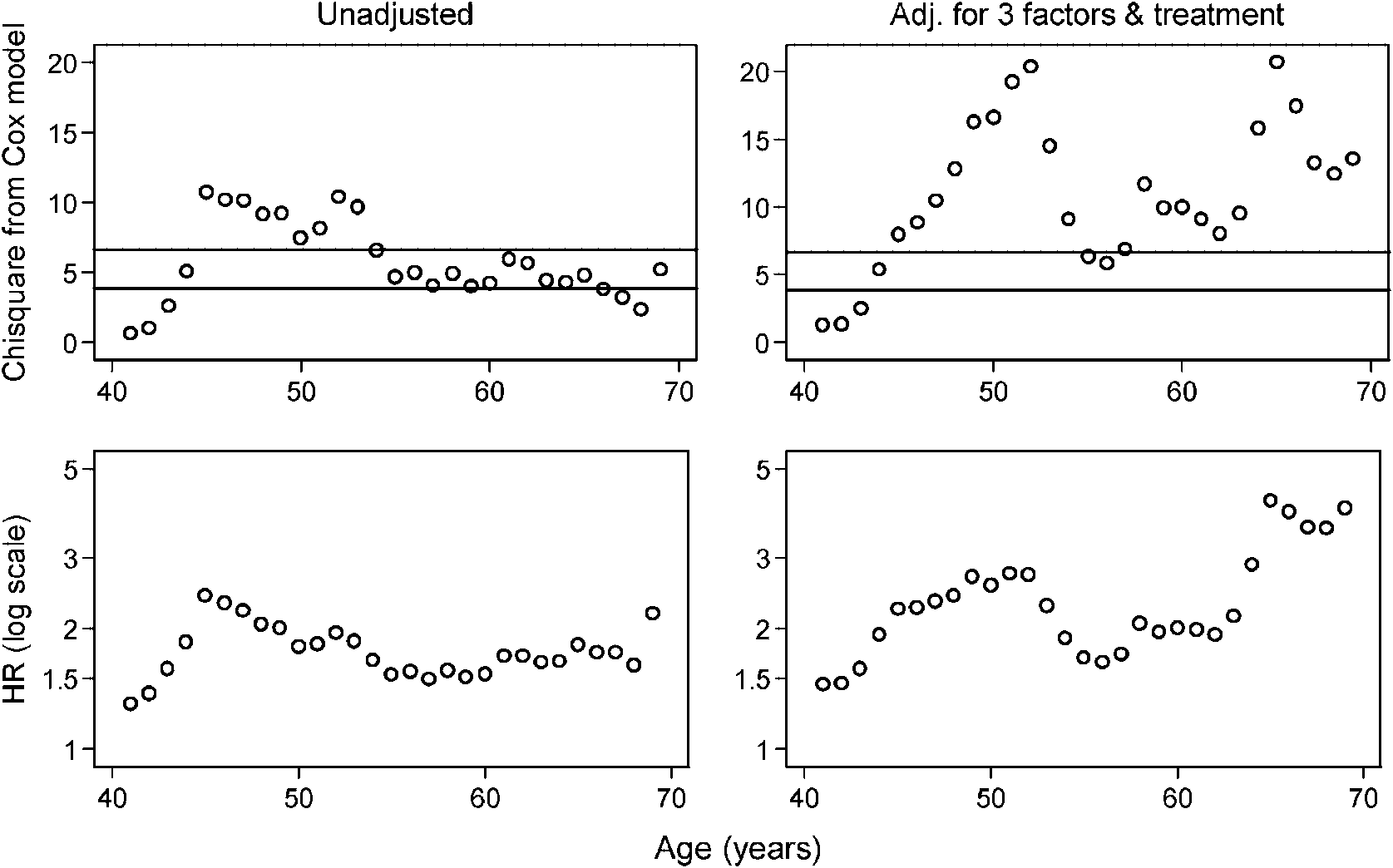
The top left panel of Figure 1 shows that the ‘optimal’ cutpoint in a univariate analysis is
at 45 years, with a 2 of about 10. After adjusting for three variables and treatment (Figure 1,top right panel) the ‘optimal’ cutpoint shifts to 65 years and has a
2 values are very unstable and are not conventionally signiÿcant for several cutpoints. Note
that 52 years is nearly as good as the ‘optimal’ cutpoint in the adjusted analysis. The estimatedHR
uctuates widely across cutpoints, particularly in the adjusted analysis (Figure 1, bottom
right panel). When the cutpoint on age is large, the risk for patients classiÿed as ‘old’ ismuch increased, but only a few patients fall into such a subgroup. For example for a cutpointof 65 years, only 14.5 per cent of patients would fall into the ‘old’ group.
Copyright ? 2005 John Wiley & Sons, Ltd.
DICHOTOMIZING CONTINUOUS PREDICTORS IN MULTIPLE REGRESSION
Figure 1. Derivation of the ‘optimal’ cutpoint for age, unadjusted (left panels) and adjusted for threeother prognostic factors and treatment (right panels). Upper panels show the
horizontal lines denoting the critical values of the
2 distribution on 1 d.f. for testing signiÿcance at
the 5 and 1 per cent levels, respectively. Lower panels show the HR for comparing ‘old’ with ‘young’
age by using dichotomization at the di erent ages shown.
3.5. Evaluation of the twofold cross-validation method
We applied Mazumdar et al.’s [24] extension of Faraggi and Simon’s [14] twofold cross-validation procedure in 50 replicates to estimate the log HR and its 95 per cent conÿdenceinterval, adjusting for three prognostic variables and treatment. A di erent random number seedwas used each time. The results are plotted ordered by the HR in Figure 2. The estimated HRhas a large variance between replicates and a positively skew distribution, making it unclearhow large the in uence of age is. The median HR is 1.8, and this may be compared with thevalue of 4.2 for the ‘optimal’ cutpoint (see Figure 1, bottom right panel).
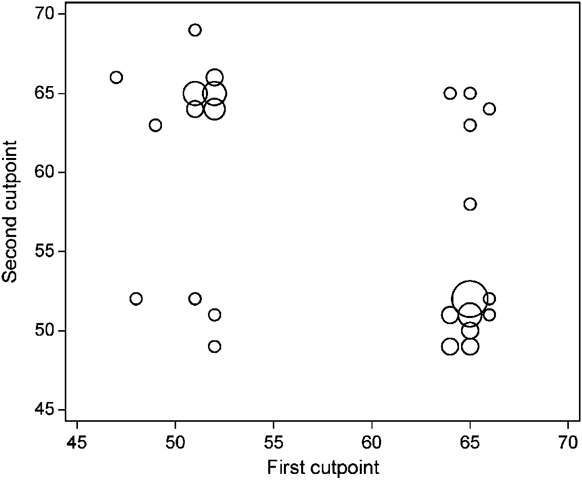
Figure 3 compares the cutpoints obtained in the two subsets across the 50 replications.
About one half of the paired cutpoints are identical. Ignoring the arbitrary ordering between‘ÿrst’ and ‘second’ cutpoints, most (41=50) of the paired cutpoints are very di erent, with onecutpoint, in the lower group, around 52 years and the other around 65 years. In only 1=50replications was the same cutpoint (65 years) chosen in both halves. It is questionable whetherestimates of HRs and P-values based on dichotomizations from such di erent cutpoints in thetwo halves have any merit.
Copyright ? 2005 John Wiley & Sons, Ltd.
P. ROYSTON, D. G. ALTMAN AND W. SAUERBREI
Figure 2. Ranked estimated HR for age in 50 replicate runs of the twofold cross-validation procedure,
with 95 per cent conÿdence intervals.
Figure 3. Pairs of ‘optimal’ cutpoints for age in random halves of the PBC data, adjusting forthree prognostic variables and treatment. The area of each circle is proportional to the number of
coincident observations plotted there.
Copyright ? 2005 John Wiley & Sons, Ltd.
DICHOTOMIZING CONTINUOUS PREDICTORS IN MULTIPLE REGRESSION
There is no obvious reason to produce a prognostic model with one or more categorizedcontinuous variables when the resulting linear predictor will still take many values. However,there is a real point in creating risk groups from such a model—not least, as an aid tomaking clinical decisions about therapy. Accordingly, we prefer ÿrst to derive a continuousrisk score from a model in which all relevant covariates are kept continuous, and then toapply categorization at the ÿnal step. Patients are divided into several groups for clinicalapplication by applying cutpoints to the risk score. Royston and Sauerbrei [28] suggest anapproach to choosing a ‘reasonable’ number of risk groups loosely based on the idea thatthe HR between neighbouring groups should be statistically signiÿcantly di erent from 1. Inthe present example, it turns out that four groups is the maximum that may be entertainedto maintain such separation of the hazard between neighbouring groups. Figure 4 showsKaplan–Meier survival curves for four groups with equal numbers of events in each, derivedfrom a risk score calculated from the MFP model. The patients separate nicely into low,low intermediate, high intermediate and high risk groups, the probability of surviving 3 yearsranging from about 25 to 90 per cent.
The PBC data originate from a randomized controlled trial of azathioprine versus placebo. In PBC, serum bilirubin concentration is a powerful predictor of survival time, and evenslight imbalance in this factor between randomized groups could induce bias in the estimatedtreatment e ect. There was indeed a small imbalance between the groups in log bilirubinof 0.23 SD units. Estimating the treatment e ect within a multivariable model is the usualapproach to adjusting for the imbalance. We assessed the robustness of the estimated treatmente ect to alternative ways of modelling the prognostic e ect of bilirubin. Table I shows the
Figure 4. Prognostic groups for PBC data based on categorizing the risk score from the MFP model. Groups 1– 4 contain 103, 39, 36 and 29 patients, respectively, with 26, 26, 27 and 26 events (deaths).
Copyright ? 2005 John Wiley & Sons, Ltd.
P. ROYSTON, D. G. ALTMAN AND W. SAUERBREI
Table I. Estimated treatment e ect in PBC data using di erent confounder models.
The strong prognostic factor bilirubin is handled di erently in each model, whereas identical adjustment forage, cirrhosis and central cholestasis is applied. See text for details.
results of the investigation with 11 di erent adjustment models. In model 1 no adjustment isapplied. In models 2–10, adjustment is done for age (linear), cirrhosis and central cholestasistogether with various transformations of bilirubin: median cutpoint (32 mmol=l), ‘optimal’univariate cutpoint (45 mmol=l), four and eight equal-sized groups, linear, quadratic, FP1, FP2and spline functions. In model 11, adjustment is by a multivariable model derived by the MFPapproach. The notation ‘FPm’ denotes a fractional polynomial function of degree m, i.e. with
m terms. The best FP1 and FP2 models for bilirubin were ÿ1 ln X and ÿ1X 0:5 + ÿ2X 0:5 ln X ,respectively. The spline model was a generalized additive model (GAM) [3] using a cubicsmoothing spline for bilirubin with four equivalent d.f. Model 1, with no adjustment, givesthe smallest estimated treatment e ect. Models 2–4, with adjustment using categorizationmodels, give HRs for comparing treatments rather closer to 1 than models 5 –11, which haveadjustment for bilirubin with many (8) groups or on a continuous scale. The treatment e ectsagree closely between models 5 and 11, even when the misspeciÿed linear function is used forbilirubin. Both cutpoint adjustment models perform quite poorly. Even four groups (model4) are not enough to abolish the e ect of the imbalance in bilirubin. The large di erencesbetween the unadjusted model and the ‘successfully’ adjusted models 5 –11 indicate that thisstudy is a rather extreme example of a trial in which randomization did not completely balancethe two treatment groups with respect to disease severity. The e ect is analogous to residualconfounding in epidemiological studies [15–17]. The unadjusted treatment e ect has a P-valueof 0.35, whereas the adjusted e ects for models 5 –11 have P-values of around 0.01.
3.8. Loss of information due to dichotomization
We compared the information content and ability to discriminate outcomes between threemodels for the PBC data. All models included the two continuous and two binary prognosticfactors identiÿed by the MFP procedure, and treatment. In model 1 both age and bilirubin weredichotomized at the median. In model 2 ‘optimal’ cutpoints, determined univariately, replacedmedian cutpoints. Model 3 was an MFP model with all continuous variables retained ascontinuous (see Section 3.3). Table II shows the model 2 statistic (calculated from di erencesin twice the log partial likelihood), c-index, D measure of separation [28] and its associated
Copyright ? 2005 John Wiley & Sons, Ltd.
DICHOTOMIZING CONTINUOUS PREDICTORS IN MULTIPLE REGRESSION
Table II. Quantifying the loss of information in two cutpoint models for the PBC data, compared
with model 3 in which continuous variables were retained as continuous.
Figure 5. Functional form of the e ect of bilirubin on the relative hazard according to the ‘op-timal’ cutpoint of 45 mmol=l (determined univariately) and three continuous models (adjusted forthree other prognostic factors and treatment). Functions are standardized such that the HR is1 at the mean bilirubin (61.9 mmol=l). The short vertical lines on the horizontal axis indicate
the values of bilirubin measurements.
R2D measure of explained variation. The increase in model 2 for the continuous model 3
compared with both cutpoint models is ¿37, and the variance explained by model 3 is muchhigher. The c-index does not show the di erences between models so clearly. The loss ofinformation due to dichotomization is slightly less with ‘optimal’ cutpoints. The estimatedtreatment e ect within models 1–3 is 0.74, 0.76 and 0.61, respectively.
It is of interest to compare a cutpoint model for bilirubin with the continuous functionsestimated by methods retaining continuous predictors as continuous. Figure 5 compares theunivariate ‘optimal’ cutpoint (45 mmol=l) with linear and spline functions, and the function(here, log) selected by MFP. Clearly, the e ect of bilirubin according to the cutpoint modelis unrealistic. Also, the associated HR of 4.2 seems greatly to underestimate the range of
Copyright ? 2005 John Wiley & Sons, Ltd.
P. ROYSTON, D. G. ALTMAN AND W. SAUERBREI
hazards seen with the continuous functions. Furthermore, none of the estimated continuousfunctions o ers any justiÿcation for the data-driven choice of 45 mmol=l as a cutpoint. Formost values of bilirubin above the mean, the straight line model probably underestimates thehazard. The MFP and spline models generally agree closely, but the spline model suggests abiologically implausible reduction in hazard for very high values of bilirubin.
It is well recognized in the methodological literature that dichotomization of continuous vari-ables introduces major problems in the analysis and interpretation of models derived in adata-dependent fashion. Nevertheless, dichotomization of continuous variables is widespreadin clinical research. Problems include loss of information, reduction in power, uncertainty indeÿning the cutpoint, arriving at a biologically implausible step function as the estimate ofa dose–response function, and the impossibility of detecting a non-monotonic dose–responserelation. Uncertainty in how to select a ‘sensible’ cutpoint to group a continuous variable intotwo classes has led researchers to use either the median or an ‘optimal’ cutpoint. The latterapproach gives a highly in ated type 1 error probability, together with biased parameter esti-mates and variances that are too small [9, 11]. Although some remedies for these di cultieshave been developed [9, 21–23], none of the authors of these papers actually recommendsthe use of ‘optimal’ cutpoints with their proposed corrections. In general, the situation seemshardly to have improved since the advice in 1993 of Maxwell and Delaney [1] to avoiddichotomization, quoted at the beginning of this paper.
Faraggi and Simon [14] put forward a method in which ‘optimal’ cutpoints are determined
in three samples (overall and in two subsamples). The cutpoint determined in the overallsample is meant to be used in general applications. These authors showed by simulation thata realistic P-value and a nearly unbiased estimate of the HR are obtained by twofold cross-validation. ‘Optimal’ cutpoints are found separately in each subset, and the cutpoint fromone subset is then used to classify patients in the other subset. Because the cutpoint used todichotomize the patients in a given subset is determined independently of these patients, theP-values and HR estimates from dichotomized data in the overall sample are claimed to beapproximately valid. Unfortunately, this ingenious idea for coping with problems in statisticalanalysis introduces fresh di culties in interpretation and general use. In 41=50 replicate runsof the procedure in the PBC study, we obtained an ‘optimal’ cutpoint for age in one subset ofabout 52 years and a corresponding value of around 65 years in the other. A patient aged 60would be classiÿed as ‘young’ in one subset and ‘old’ in the other. The ‘optimal’ cutpoint inthe overall sample is 65, but the
2 value for the cutpoint 52 is nearly as large (20.3 versus
Recently, Mazumdar et al. [24] extended Faraggi and Simon’s approach by ÿnding the
‘optimal’ cutpoint for a variable of interest in a multivariable setting with adjustment forother factors. Assuming an underlying cutpoint model and a multivariate correlation structurebetween several continuous variables, they showed by simulation that the power was increasedand estimates of the HR and the cutpoint were less biased when compared with the univariateapproach. They also compared it with a split-sample approach. In the latter, an ‘optimal’cutpoint is determined in a 50 per cent random subsample and used to classify patients inthe complementary half. Compared with cross-validation, the split-sample method had lower
Copyright ? 2005 John Wiley & Sons, Ltd.
DICHOTOMIZING CONTINUOUS PREDICTORS IN MULTIPLE REGRESSION
power and more biased estimates of the HR and cutpoint. The ÿndings are as expected, sincein the split-sample method, the sample size for the estimates and tests is reduced by half(see Reference [29] for further arguments against such an approach). Unfortunately, Mazumdaret al. [24] do not mention how to deÿne the multivariable model. In an example in whichidentiÿcation of a group of patients at high risk of relapse from prostate cancer was required,they note that the search for a cutpoint for lactate dehydrogenase (LDH) gave di erent resultsin the univariate and multivariable settings. In the penultimate sentence of their paper, theystress that ‘to incorporate the new markers in the decision-making process, categorizationof these variables is essential’. We feel that this statement contradicts their own simulationresults in which they demonstrate a substantial loss of power when a cutpoint model is usedin cases where a smooth relationship exists between a continuous covariate and the outcome.
Instead of dichotomizing a continuous variable, we prefer to obtain a prognostic index by
methodology which combines selection of variables with selection of functions for continuousvariables [4, 26]. As stated in an editorial [2] in an epidemiological journal a decade ago, ‘theseelegant approaches [fractional polynomials and splines] merit a larger role in epidemiology.’Clinical researchers should in general avoid dichotomization at the model-building stage andadopt more powerful methods. In our analysis of the data from the PBC study, we comparedseveral di erent approaches to creating a prognostic index. Explained variation was smallestfor the model based on the median cutpoint, 6 per cent higher for the index derived withthe ‘optimal’ cutpoint and 31 per cent higher for the MFP model. Although these ÿgureswill be slight over-estimates because no allowance has been made for data-dependent model-building, the advantage of using full information is obvious. We agree that medical decision-making often requires categorization of data, e.g. to deÿne a high-risk group of patients fora clinical trial, as in Reference [24] example. However, categorization should be appliedto the prognostic index, not to the original prognostic variables. Not to do so risks a lossof discrimination through ine cient use of the full information available with a continuousprognostic index.
By estimating the treatment e ect in the PBC data within di erent adjustment models, we
showed that the method used to adjust for an unbalanced, strongly prognostic variable can in-
uence the result. Adjustment for bilirubin dichotomized at the median cutpoint does not fully
correct for imbalance. Epidemiologists would state that there was residual confounding. Useof more groups or the full information from the continuous variable further reduces residualconfounding and results in larger estimates of the treatment e ect. This ÿnding agrees withsimulation studies in the epidemiological literature on the ability to reduce residual confound-ing by categorized variables [15, 17, 30]. Brenner and Blettner [17] state that ‘inclusion of theconfounder as a single linear term often provides satisfactory control for confounding evenin situations in which the model assumptions are clearly violated. In contrast, categorizationof the confounder may often lead to serious residual confounding if the number of categoriesis small.’ The most extreme situation of two categories seems to have been abandoned inepidemiological studies.
For model building with continuous data, software is available for methods such as mul-
tivariable fractional polynomials [31, 32] and GAMs (e.g. in S-plus and R). Royston andSauerbrei [33] demonstrated in a detailed resampling study that over-ÿtting and the resultinginstability need not be a serious issue with MFP models. Even the use of conventional polyno-mials would in general improve on dichotomization. These methods should replace analysesusing dichotomized continuous variables. Preference for one particular approach should be
Copyright ? 2005 John Wiley & Sons, Ltd.
P. ROYSTON, D. G. ALTMAN AND W. SAUERBREI
guided by parsimony, an important criterion for selecting the simplest adequate descriptor ofa functional form [2].
We are grateful for the support provided by the Volkswagen-Stiftung (RiP-program) at the Mathema-tisches Forschungsinstitut, Oberwolfach, Germany. Some of the work was carried out at Oberwolfachduring a visit in 2004.
1. Maxwell SE, Delaney HD. Bivariate median-splits and spurious statistical signiÿcance. Psychological Bulletin
2. Weinberg CR. How bad is categorization? Epidemiology 1995; 6:345 –347. 3. Hastie TJ, Tibshirani RJ. Generalized Additive Models. Chapman & Hall: New York, 1990. 4. Royston P, Altman DG. Regression using fractional polynomials of continuous covariates: parsimonious
parametric modelling (with discussion). Applied Statistics 1994; 43(3):429 – 467.
5. Del Priore G, Zandieh P, Lee MJ. Treatment of continuous data as categoric variables in obstetrics and
gynecology. Obstetrics and Gynecology 1997; 89:351–354.
6. MacCallum RC, Zhang S, Preacher KJ, Rucker DD. On the practice of dichotomization of quantitative variables.
Psychological Methods 2002; 7:19 – 40.
7. Irwin JR, McClelland GH. Negative consequences of dichotomizing continuous predictor variables. Journal of
Marketing Research 2003; 40:366 –371.
8. Cohen J. The cost of dichotomization. Applied Psychological Measurement 1983; 7:249 –253. 9. Altman DG, Lausen B, Sauerbrei W, Schumacher M. The dangers of using ‘optimal’ cutpoints in the evaluation
of prognostic factors. Journal of the National Cancer Institute 1994; 86:829 – 835.
10. Harrell Jr FE. Problems caused by categorizing continuous variables. http:==biostat.mc.vanderbilt.edu=twiki=bin=
view=Main=CatContinuous, 2004. Accessed on 6.9.2004.
11. Austin PC, Brunner LJ. In ation of the type I error rate when a continuous confounding variable is categorized
in logistic regression analyses. Statistics in Medicine 2004; 23:1159 –1178.
12. Lagakos SW. E ects of mismodelling and mismeasuring explanatory variables on tests of their association with
a response variable. Statistics in Medicine 1988; 7:257 –274.
13. Breslow NE, Day NE. Statistical Methods in Cancer Research, vol. 1. IARC Scientiÿc Publications: Lyon,
14. Faraggi D, Simon R. A simulation study of cross-validation for selecting an optimal cutpoint in univariable
survival analysis. Statistics in Medicine 1996; 15:2203 –2213.
15. Becher H. The concept of residual confounding in regression models and some applications. Statistics in
16. Cochran WG. The e ectiveness of adjustment by subclassiÿcation in removing bias in observational studies.
17. Brenner H, Blettner M. Controlling for continuous confounders in epidemiologic research. Epidemiology 1997;
18. Wartenberg D, Northridge M. Deÿning exposure in case-control studies: a new approach. American Journal of
Epidemiology 1991; 133:1058 –1071.
19. Miller R, Siegmund D. Maximally selected chi-square statistics. Biometrics 1982; 38:1011–1016. 20. Lausen B, Schumacher M. Evaluating the e ect of optimized cuto
factors. Computational Statistics and Data Analysis 1996; 21:307 –326.
21. Hilsenbeck SG, Clark GM. Practical P-value adjustment for optimally selected cutpoints. Statistics in Medicine
22. Schumacher M, Hollander N, Sauerbrei W. Resampling and cross-validation techniques: a tool to reduce bias
caused by model-building? Statistics in Medicine 1997; 16:2813 –2827.
23. Hollander N, Sauerbrei W, Schumacher M. Conÿdence intervals for the e ect of a prognostic factor after
selection of an ‘optimal’ cutpoint. Statistics in Medicine 2004; 23:1701–1713.
24. Mazumdar M, Smith A, Bacik J. Methods for categorizing a prognostic variable in a multivariable setting.
Statistics in Medicine 2003; 22:559 –571.
25. Christensen E, Neuberger J, Crowe J, Altman DG, Popper H, Portmann B, Doniach D, Ranek L. Tygstrup
N, Williams R. Beneÿcial e ect of azathioprine and prediction of prognosis in primary biliary cirrhosis: ÿnalresults of an international trial. Gastroenterology 1985; 89:1084 –1091.
Copyright ? 2005 John Wiley & Sons, Ltd.
DICHOTOMIZING CONTINUOUS PREDICTORS IN MULTIPLE REGRESSION
26. Sauerbrei W, Royston P. Building multivariable prognostic and diagnostic models: transformation of the
predictors by using fractional polynomials. Journal of the Royal Statistical Society Series A 1999; 162:71–94(Corrigendum: Journal of the Royal Statistical Society, Series A 2002; 165:399 – 400).
27. Royston P, Sauerbrei W. A new approach to modelling interactions between treatment and continuous covariates
in clinical trials by using fractional polynomials. Statistics in Medicine 2004; 23:2509 –2525.
28. Royston P, Sauerbrei W. A new measure of prognostic separation in survival data. Statistics in Medicine 2004;
29. Hirsch RP. Validation samples. Biometrics 1991; 47:1193 –1194. 30. Greenland S. Avoiding power loss associated with categorization and ordinal scores in dose-response and trend
analysis. Epidemiology 1995; 6:450 – 454.
31. StataCorp. Stata Reference Manual, Version 8. Stata Press: College Station, TX, 2003. 32. Sauerbrei W, Meier-Hirmer C, Benner A, Royston P. Multivariable regression model building by using fractional
polynomials: description of SAS, Stata and R programs. Computational Statistics and Data Analysis, 2005,submitted.
33. Royston P, Sauerbrei W. Stability of multivariable fractional polynomial models with selection of variables and
transformations: a bootstrap investigation. Statistics in Medicine 2003; 22:639 – 659.
Copyright ? 2005 John Wiley & Sons, Ltd.
Yes, the third term has now arrived; my how the year passes. Because of the large number of deadlines and that only one and a half weeks of this term make up April, we are going light on events. This also means having too many deadlines is no excuse!As you all know, your wonderful committee has put a lot of effort into making the society the best it can be this past year. In fact, this effort
DELPROV 9 Delprovet innehåller 20 uppgifter. Anvisningar Delprovet LÄS prövar din förmåga att ta till dig innehållet i texter skrivna på svenska. Provet består av fem texter från olika ämnesområden. Till varje text hör fyra uppgifter. Varje uppgift består av en fråga med fyra svarsförslag. Ett av svarsförslagen är rätt. Läs texten och välj ut det svarsförslag som m
 DICHOTOMIZING CONTINUOUS PREDICTORS IN MULTIPLE REGRESSION
Figure 1. Derivation of the ‘optimal’ cutpoint for age, unadjusted (left panels) and adjusted for threeother prognostic factors and treatment (right panels). Upper panels show the
horizontal lines denoting the critical values of the
2 distribution on 1 d.f. for testing signiÿcance at
the 5 and 1 per cent levels, respectively. Lower panels show the HR for comparing ‘old’ with ‘young’
age by using dichotomization at the di erent ages shown.
DICHOTOMIZING CONTINUOUS PREDICTORS IN MULTIPLE REGRESSION
Figure 1. Derivation of the ‘optimal’ cutpoint for age, unadjusted (left panels) and adjusted for threeother prognostic factors and treatment (right panels). Upper panels show the
horizontal lines denoting the critical values of the
2 distribution on 1 d.f. for testing signiÿcance at
the 5 and 1 per cent levels, respectively. Lower panels show the HR for comparing ‘old’ with ‘young’
age by using dichotomization at the di erent ages shown.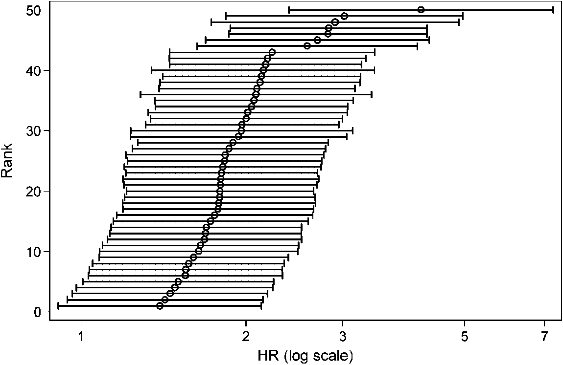
 P. ROYSTON, D. G. ALTMAN AND W. SAUERBREI
Figure 2. Ranked estimated HR for age in 50 replicate runs of the twofold cross-validation procedure,
with 95 per cent conÿdence intervals.
P. ROYSTON, D. G. ALTMAN AND W. SAUERBREI
Figure 2. Ranked estimated HR for age in 50 replicate runs of the twofold cross-validation procedure,
with 95 per cent conÿdence intervals.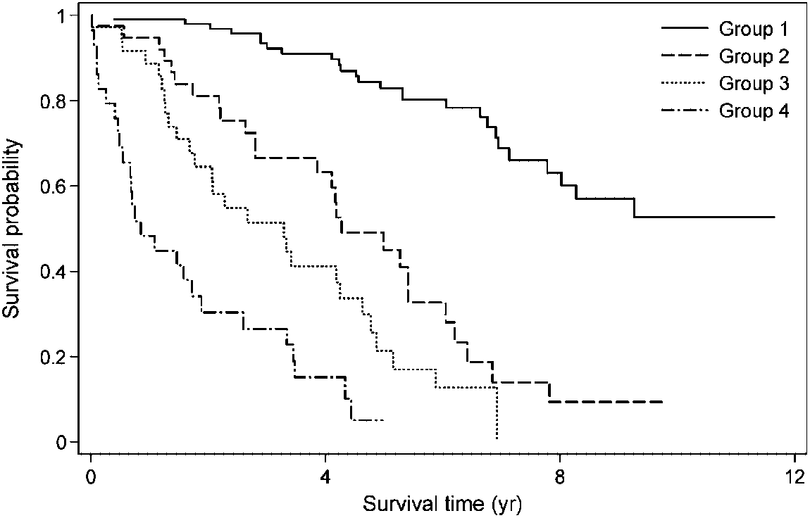 DICHOTOMIZING CONTINUOUS PREDICTORS IN MULTIPLE REGRESSION
There is no obvious reason to produce a prognostic model with one or more categorizedcontinuous variables when the resulting linear predictor will still take many values. However,there is a real point in creating risk groups from such a model—not least, as an aid tomaking clinical decisions about therapy. Accordingly, we prefer ÿrst to derive a continuousrisk score from a model in which all relevant covariates are kept continuous, and then toapply categorization at the ÿnal step. Patients are divided into several groups for clinicalapplication by applying cutpoints to the risk score. Royston and Sauerbrei [28] suggest anapproach to choosing a ‘reasonable’ number of risk groups loosely based on the idea thatthe HR between neighbouring groups should be statistically signiÿcantly di erent from 1. Inthe present example, it turns out that four groups is the maximum that may be entertainedto maintain such separation of the hazard between neighbouring groups. Figure 4 showsKaplan–Meier survival curves for four groups with equal numbers of events in each, derivedfrom a risk score calculated from the MFP model. The patients separate nicely into low,low intermediate, high intermediate and high risk groups, the probability of surviving 3 yearsranging from about 25 to 90 per cent.
DICHOTOMIZING CONTINUOUS PREDICTORS IN MULTIPLE REGRESSION
There is no obvious reason to produce a prognostic model with one or more categorizedcontinuous variables when the resulting linear predictor will still take many values. However,there is a real point in creating risk groups from such a model—not least, as an aid tomaking clinical decisions about therapy. Accordingly, we prefer ÿrst to derive a continuousrisk score from a model in which all relevant covariates are kept continuous, and then toapply categorization at the ÿnal step. Patients are divided into several groups for clinicalapplication by applying cutpoints to the risk score. Royston and Sauerbrei [28] suggest anapproach to choosing a ‘reasonable’ number of risk groups loosely based on the idea thatthe HR between neighbouring groups should be statistically signiÿcantly di erent from 1. Inthe present example, it turns out that four groups is the maximum that may be entertainedto maintain such separation of the hazard between neighbouring groups. Figure 4 showsKaplan–Meier survival curves for four groups with equal numbers of events in each, derivedfrom a risk score calculated from the MFP model. The patients separate nicely into low,low intermediate, high intermediate and high risk groups, the probability of surviving 3 yearsranging from about 25 to 90 per cent.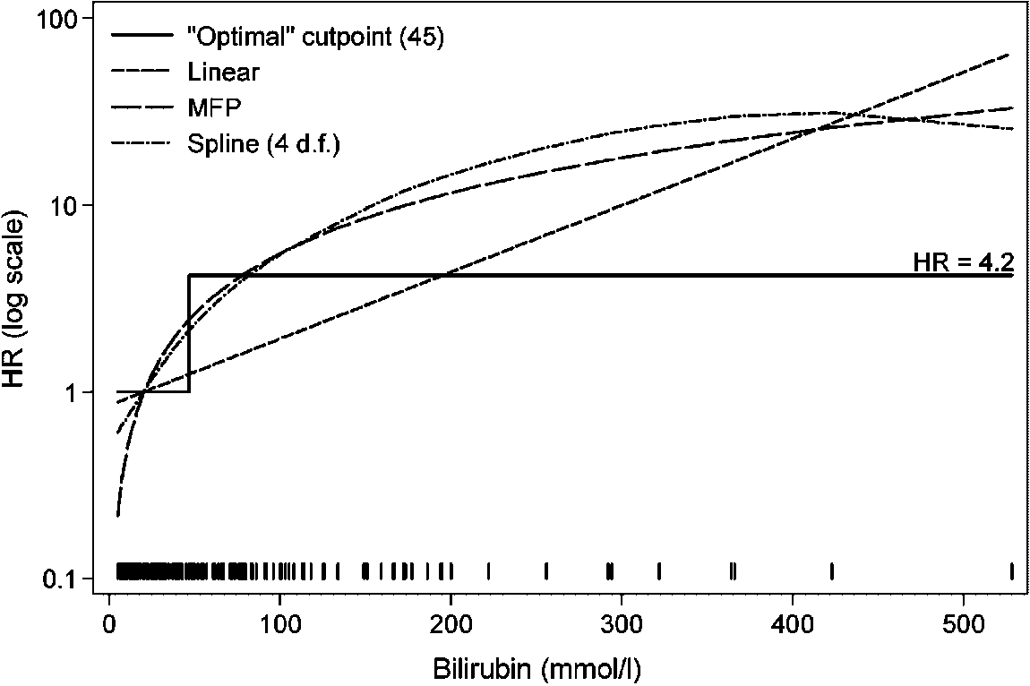 DICHOTOMIZING CONTINUOUS PREDICTORS IN MULTIPLE REGRESSION
Table II. Quantifying the loss of information in two cutpoint models for the PBC data, compared
with model 3 in which continuous variables were retained as continuous.
DICHOTOMIZING CONTINUOUS PREDICTORS IN MULTIPLE REGRESSION
Table II. Quantifying the loss of information in two cutpoint models for the PBC data, compared
with model 3 in which continuous variables were retained as continuous.